Extreme Fill 2D

May 7, 2013

Introduction

The extreme fill 1D model has been extended to 2D. Although, the 1D model uses transient terms for all the equations, the electrode/electrolyte interface is held in a stationary position. This idealized system helps explain the most puzzling aspect of extreme fill, the initial formation of the “on” and “off” states of deposition (see previous blog post. While the 1D model captures the most important qualitative aspect of extreme fill, it is not particularly accurate for making fill/fail predictions. The 2D extreme fill model aims to improve the accuracy by using the level set method to model the moving interface in similar way to the old 2D superfill models, but now uses the new level set implementation recently introduced into FiPy. The extreme fill 2D model is hosted at Github.

Note on IPython and Jekyll

This is a just a note on integrating the IPython notebook into the Jekyll blog. The blog post by David Ketcheson includes a script to automate the IPython to Jekyll transition. The script has been modified for my own needs (see the script on Github). There are a number of issues that aren’t yet ironed out such as embedding Sumatra markdown tables rather than HTML and including hover text with Sumatra labels for figures.

Demonstration

As a demonstration of the model, a movie has been made from the following Sumatra record. This also demonstrates embedding a Sumatra table in IPython.

from smtext import getSMTRecords, smt_ipy_table
records = getSMTRecords(tags=['serialnumber18'],parameters={'Nx' : 600})
smt_ipy_table(records, fields=['label', 'timestamp', 'parameters', 'repository', 'version'], parameters=['Nx'])

Label	Timestamp	Parameters	Repository	Version
`58d17d49efd8`	2013-04-26 17:55	`Nx: 600`	`git@github.com:wd15/extremefill-data.git`	`a4e17af0c25a`

Convergence

The following sections contain a rudimentary $\chi$ -by-eye convergence analysis. Further convergence testing may be done, but it is probably best to actually produce some useful results and revisit convergence when the model is closer to being finalized.

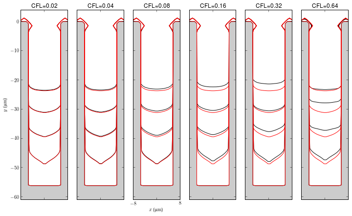
CFL Number

The figures show convergence as the CFL decreases from 0.64 to 0.01. The contours presented are for the time steps that have the closest elapsed times to the times argument (time step size is not uniform for these simulations). The red contour is for CFL=0.01 (the base case).

from multiViewer import MultiViewer
from smtext import getSMTRecords, smt_ipy_table

records = getSMTRecords(tags=['CFL', 'production'])
records = [getSMTRecords(records=records, parameters={'CFL' : CFL})[0] for CFL in (0.01, 0.02, 0.04, 0.08, 0.16, 0.32, 0.64)]
title = [r'CFL={0:1.2f}'.format(r.parameters['CFL']) for r in records[1:]]
viewer = MultiViewer(records[1:], baseRecords=records[0], title=title, figsize=(12, 9))
viewer.plot(times=(0., 1000., 2000., 3000., 4000.))
smt_ipy_table(records, fields=['label', 'timestamp', 'parameters', 'repository', 'version', 'duration'], parameters=['CFL'])

Label	Timestamp	Parameters	Repository	Version	Duration
`76cc1cca1d89`	2013-02-22 13:40	`CFL: 0.01`	`git@github.com:wd15/extremefill-data.git`	`0e0334ae83ae`	6h 9m 0.42s
`e07c8a307a1e`	2013-02-22 13:40	`CFL: 0.02`	`git@github.com:wd15/extremefill-data.git`	`0e0334ae83ae`	3h 41m 14.56s
`678975cf7009`	2013-02-22 13:40	`CFL: 0.04`	`git@github.com:wd15/extremefill-data.git`	`0e0334ae83ae`	2h 19m 31.04s
`a9431ee7da68`	2013-02-21 16:32	`CFL: 0.08`	`git@github.com:wd15/extremefill-data.git`	`0592f3835b5c`	1h 18m 11.83s
`9f933d3ae816`	2013-02-21 16:32	`CFL: 0.16`	`git@github.com:wd15/extremefill-data.git`	`0592f3835b5c`	43m 40.75s
`36f7e8fa0702`	2013-02-21 16:32	`CFL: 0.32`	`git@github.com:wd15/extremefill-data.git`	`0592f3835b5c`	24m 44.49s
`a1e3ead836eb`	2013-02-21 16:32	`CFL: 0.64`	`git@github.com:wd15/extremefill-data.git`	`0592f3835b5c`	17m 53.83s

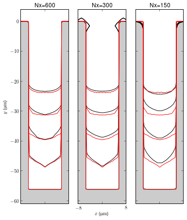
Grid Spacing

The figures show a comparison between Nx=1200 (the red curves) and Nx=150, 300, 600. Nx is the total number of cells from the bottom to the top of the domain including the length of the feature and the boundary layer. The results do not demonstrate any clear grid convergence at present and further results with finer grids are required. These runs are all in serial at present. Some changes are required to the level set implementation in FiPy to run in parallel to allow comparison with finer grids.

from multiViewer import MultiViewer
from smtext import getSMTRecords, smt_ipy_table

records = getSMTRecords(tags=['batch2'])
records = [getSMTRecords(records=records, parameters={'Nx' : Nx})[0] for Nx in (1200, 600, 300, 150)]
title = [r'Nx={0:d}'.format(r.parameters['Nx']) for r in records[1:]]
viewer = MultiViewer(records[1:], baseRecords=records[0], title=title, figsize=(6, 9))
viewer.plot(times=(0., 1000., 2000., 3000., 4000.))
smt_ipy_table(records, fields=['label', 'timestamp', 'parameters', 'repository', 'version', 'duration'], parameters=['Nx'])

Label	Timestamp	Parameters	Repository	Version	Duration
`143dec5e7ecd`	2013-02-28 11:48	`Nx: 1200`	`git@github.com:wd15/extremefill-data.git`	`81f76189d481`	5d 21h 57m 20.14s
`4282f5340892`	2013-02-28 11:51	`Nx: 600`	`git@github.com:wd15/extremefill-data.git`	`81f76189d481`	11h 8m 2.38s
`e66ca6267686`	2013-02-28 11:48	`Nx: 300`	`git@github.com:wd15/extremefill-data.git`	`81f76189d481`	1h 26m 11.63s
`85626d5b2715`	2013-02-28 11:51	`Nx: 150`	`git@github.com:wd15/extremefill-data.git`	`81f76189d481`	16m 39.49s

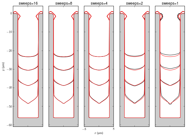
Sweeps

from multiViewer import MultiViewer
from smtext import getSMTRecords, smt_ipy_table

records = getSMTRecords(tags=['serialnumber4'])
records = [getSMTRecords(records=records, parameters={'sweeps' : sweeps})[0] for sweeps in (32, 16, 8, 4, 2, 1)]
title = [r'sweeps={0:d}'.format(r.parameters['sweeps']) for r in records[1:]]
viewer = MultiViewer(records[1:], baseRecords=records[0], title=title, figsize=(10, 9))
viewer.plot(times=(0., 1000., 2000., 3000., 4000.))
smt_ipy_table(records, fields=['label', 'timestamp', 'parameters', 'repository', 'version', 'duration'], parameters=['sweeps'])

Label	Timestamp	Parameters	Repository	Version	Duration
`7ed71a0a1faf`	2013-03-26 17:12	`sweeps: 32`	`git@github.com:wd15/extremefill-data.git`	`26a1c53dc79c`	3h 35m 47.96s
`7a17de0b7487`	2013-03-26 17:12	`sweeps: 16`	`git@github.com:wd15/extremefill-data.git`	`26a1c53dc79c`	3h 10m 54.34s
`8307dc417ea0`	2013-03-26 17:12	`sweeps: 8`	`git@github.com:wd15/extremefill-data.git`	`26a1c53dc79c`	1h 6m 16.29s
`e16fa2b84942`	2013-03-26 17:12	`sweeps: 4`	`git@github.com:wd15/extremefill-data.git`	`26a1c53dc79c`	1h 3m 56.60s
`528f07e88fae`	2013-03-26 17:12	`sweeps: 2`	`git@github.com:wd15/extremefill-data.git`	`26a1c53dc79c`	26m 3.20s
`331ce2cd522c`	2013-03-26 17:12	`sweeps: 1`	`git@github.com:wd15/extremefill-data.git`	`26a1c53dc79c`	15m 42.37s

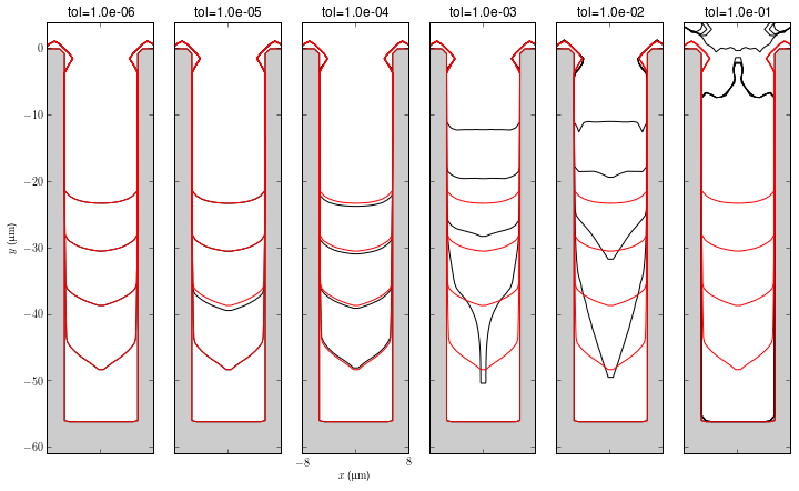
Linear Tolerance

from multiViewer import MultiViewer
from smtext import getSMTRecords, smt_ipy_table

records = getSMTRecords(tags=['serialnumber7'])
records = [getSMTRecords(records=records, parameters={'solver_tol' : solver_tol})[0] for solver_tol in (1e-7, 1e-6, 1e-5, 1e-4, 1e-3, 1e-2, 1e-1)]
title = [r'tol={0:1.1e}'.format(r.parameters['solver_tol']) for r in records[1:]]
viewer = MultiViewer(records[1:], baseRecords=records[0], title=title, figsize=(12, 9))
viewer.plot(times=(0., 1000., 2000., 3000., 4000.))
smt_ipy_table(records, fields=['label', 'timestamp', 'parameters', 'repository', 'version', 'duration'], parameters=['solver_tol'])

Label	Timestamp	Parameters	Repository	Version	Duration
`faa5d9f206ed`	2013-03-27 11:25	`solver_tol: 1e-07`	`git@github.com:wd15/extremefill-data.git`	`a5790e469d66`	32m 58.14s
`f59dfdbec834`	2013-03-27 11:24	`solver_tol: 1e-06`	`git@github.com:wd15/extremefill-data.git`	`a5790e469d66`	33m 43.28s
`9bc8c7395961`	2013-03-27 11:24	`solver_tol: 1e-05`	`git@github.com:wd15/extremefill-data.git`	`a5790e469d66`	31m 14.05s
`417bcf854132`	2013-03-27 11:24	`solver_tol: 0.0001`	`git@github.com:wd15/extremefill-data.git`	`a5790e469d66`	27m 41.94s
`33b8c8063ac2`	2013-03-27 11:24	`solver_tol: 0.001`	`git@github.com:wd15/extremefill-data.git`	`a5790e469d66`	25m 56.36s
`5ad7bdc1a530`	2013-03-27 11:24	`solver_tol: 0.01`	`git@github.com:wd15/extremefill-data.git`	`a5790e469d66`	31m 59.05s
`2531d84308b4`	2013-03-27 11:24	`solver_tol: 0.1`	`git@github.com:wd15/extremefill-data.git`	`a5790e469d66`	1h 6m 29.66s

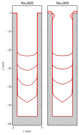
Control Parameters

Using the images above, the control parameters will be adjusted from

sweeps = 30
solver_tol = 1e-6
CFL = 0.1
tol = 1e-1```

to

sweeps = 4 solver_tol = 1e-10 CFL = 0.1 tol = 1e-10```

Using these new parameters, simulations have been run with Nx=150, 300, 600 and compared with the old parameters. Simulations with the new parameters are more efficient without sacrificing accuracy.

from multiViewer import MultiViewer
from smtext import getSMTRecords, smt_ipy_table

Nxs = (600, 300)
records = getSMTRecords(tags=['serialnumber8'])
records = [getSMTRecords(records=records, parameters={'Nx' : Nx})[0] for Nx in Nxs]
baseRecords = getSMTRecords(tags=['batch2'])
baseRecords = [getSMTRecords(records=baseRecords, parameters={'Nx' : Nx})[0] for Nx in Nxs]
title = [r'Nx={0:d}'.format(r.parameters['Nx']) for r in records]
viewer = MultiViewer(records, baseRecords=baseRecords, title=title, figsize=(4, 9))
viewer.plot(times=(0., 1000., 2000., 3000., 4000.))
smt_ipy_table(records + baseRecords, fields=['label', 'timestamp', 'parameters', 'repository', 'version', 'duration'], parameters=['Nx'])

Label	Timestamp	Parameters	Repository	Version	Duration
`d83505552902`	2013-03-27 14:22	`Nx: 600`	`git@github.com:wd15/extremefill-data.git`	`a5790e469d66`	4h 20m 30.13s
`8cdf3a35f80f`	2013-03-27 14:22	`Nx: 300`	`git@github.com:wd15/extremefill-data.git`	`a5790e469d66`	28m 45.72s
`4282f5340892`	2013-02-28 11:51	`Nx: 600`	`git@github.com:wd15/extremefill-data.git`	`81f76189d481`	11h 8m 2.38s
`e66ca6267686`	2013-02-28 11:48	`Nx: 300`	`git@github.com:wd15/extremefill-data.git`	`81f76189d481`	1h 26m 11.63s